← All work — 2025-26

RP3: TVC Landing Simulation

Landing a thrust-vector-controlled sounding rocket after main-chute deployment: a 3-DOF Simulink simulation, a phased LQR controller and a 300-run Monte-Carlo campaign.

RoleYear-3 individual research project, supervised by Prof. Tom Richardson

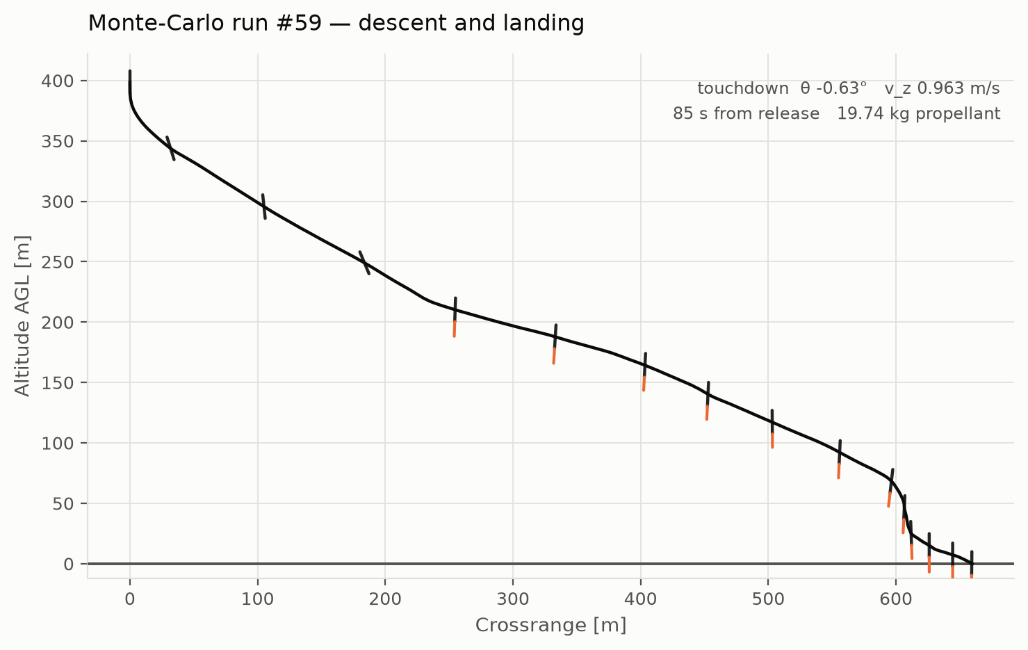
Descent and landing of Monte-Carlo run 59: altitude above ground against crossrange, the vehicle drawn at its own logged attitude every few seconds with the plume shown where thrust is commanded, flaring to touchdown 660 m downrange — Run #59 flown from its own log: 398 m and 40 m/s at release to θ −0.63° and v_z 0.963 m/s at touchdown, 85 s later.

Monte-Carlo success

209/300

Best landing pitch

−0.63°

Mean propellant

12.6 kg

Land a rocket after the chute

My Year-3 research project (AENG30017), supervised by Prof. Tom Richardson: land a sounding rocket softly and upright after it has already come down under its main chute. The vehicle descends at about 8 m/s; at 200 m a phased LQR and thrust-vector-control system arrests the wind-driven pendulum swing and flies the last 25 seconds to touchdown. If the controller fails, the rocket keeps riding the chute, a survivable parachute landing rather than a lost vehicle. The plant is a 3-DOF MATLAB/Simulink model of a 78 kg, 3.97 m, 20:1-fineness airframe (HyPower's Waxwing) with a hypothetical deep-throttle 5 kN LOx-class engine, Isp 180 s, gimbal ±10°.

Cutaway render of the slender Waxwing sounding-rocket airframe lying horizontally, fins at the left and red nose section at the right — Waxwing airframe cutaway: 3.97 m by 0.2 m diameter, 20:1 fineness.

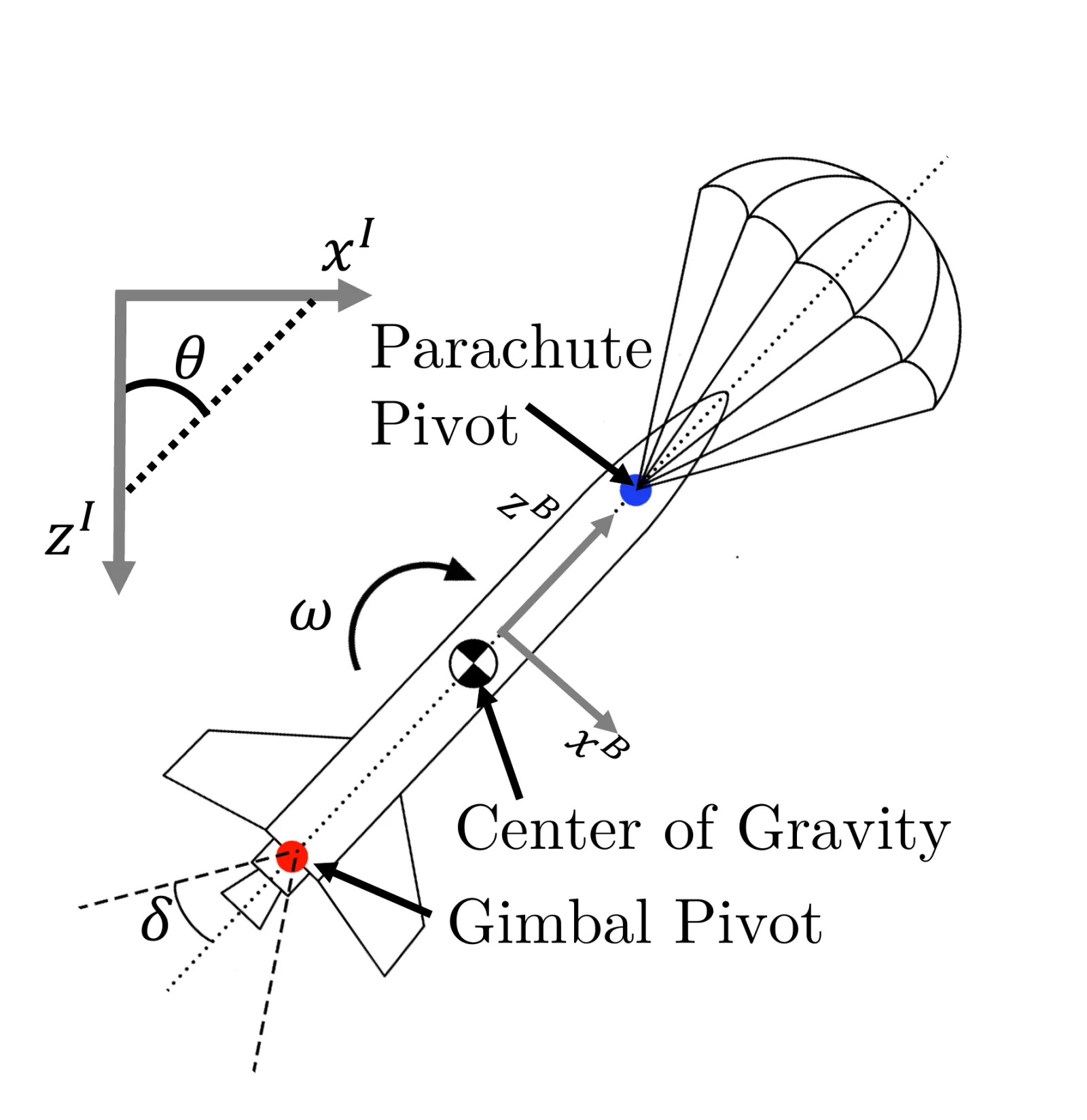
Line diagram of a tilted rocket hanging under a parachute, marking the parachute pivot, centre of gravity and gimbal pivot, with the inertial and body frames and the angles theta, omega and delta — Frames and geometry: inertial frame z-down, body frame at the centre of gravity, engine at the gimbal pivot. θ and δ as used throughout.

The controller

Four gates, three modes. The controller arms at 200 m and runs three LQR modes in phase: damping to kill the swing, stabilisation to hold the vehicle vertical once it is calm, and a flare from 25 m targeting 1.8 m/s. Each mode carries dynamic lead compensation (τ 0.12-0.22 s) to cover the engine lag and rate limits, which I fitted to BristolSEDS hotfire data. Two safety layers sit on top. Predictive recovery cuts thrust above |θ| 50° or |ω| 160°/s and lets the chute re-right the vehicle before the controller re-engages; an emergency max-thrust override is the last resort. The passive plant it fights has ω_n 4.264 rad/s and ζ ≈ 0.014, so a 19° swing takes 45 s to decay below 2° on its own.

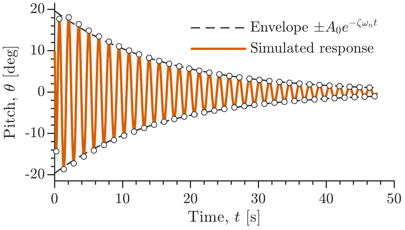
Pitch angle oscillating between plus and minus 19 degrees and decaying over 45 seconds inside a fitted exponential envelope — Passive aerodynamic damping: 19° to under 2° in 45 s. ω_n 4.264 rad/s, ζ ≈ 0.014.

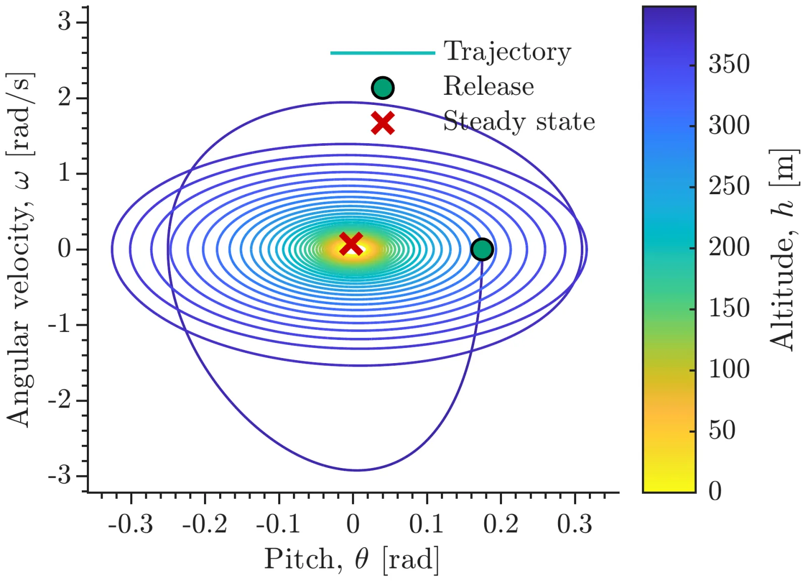
Angular velocity against pitch for the passive descent, a spiral of ellipses coloured from blue at release to yellow near the ground, contracting onto the steady-state point — Passive ω-θ phase portrait coloured by altitude: a contracting spiral, no limit cycles.

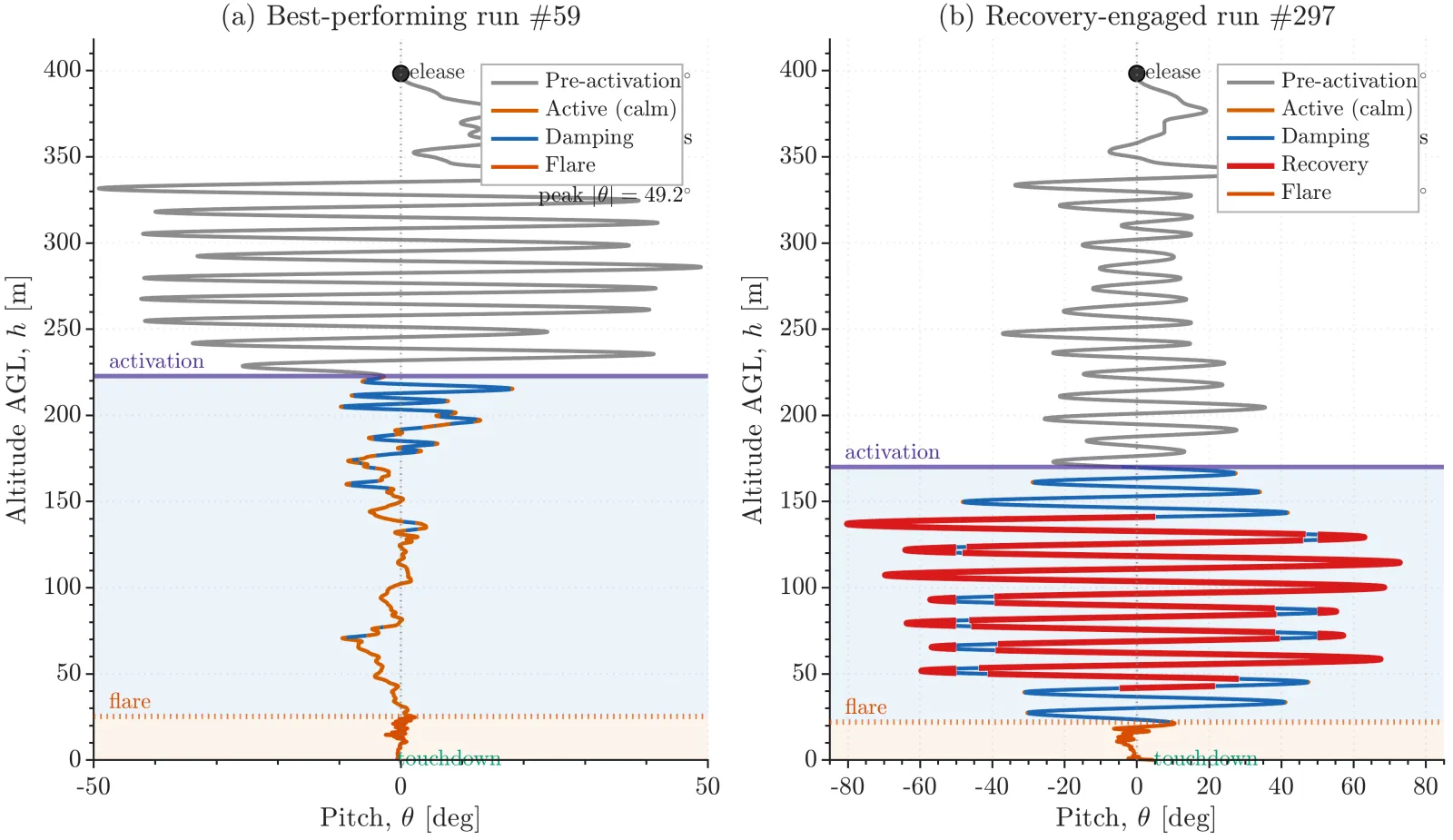
Two altitude-against-pitch plots side by side: the best run settles to near-zero pitch soon after activation at 200 m, while the recovery-engaged run swings to plus and minus 80 degrees in red before the controller re-engages and lands — Best run #59 beside recovery-engaged run #297: thrust cut, the chute re-rights the vehicle, the controller re-engages and still lands.

Three hundred runs

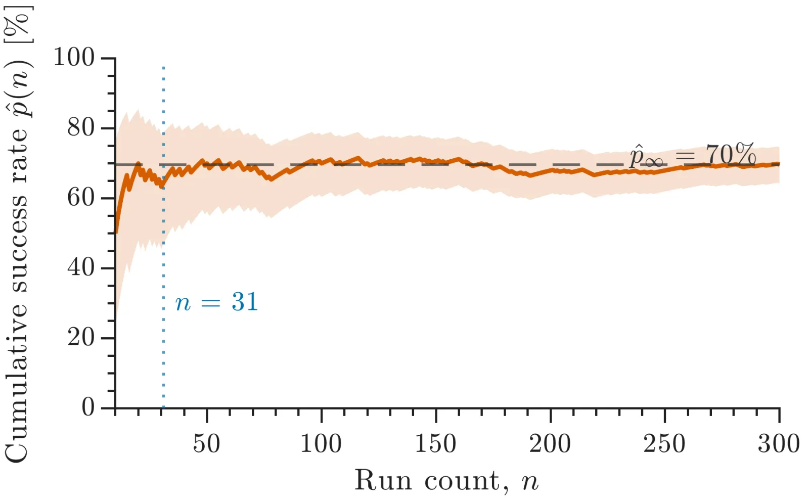
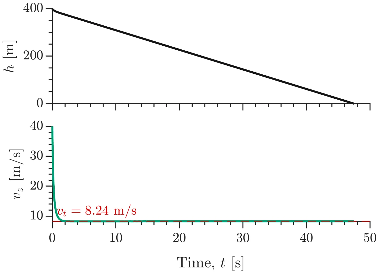
Wind shear, gusts and Dryden turbulence are random, so one landing proves nothing. I ran 300 Monte-Carlo descents with the L controller. 209 landed inside the success box of |v_z| below 3 m/s and |θ| below 5° at touchdown, 22 landed out of spec and 69 spun: 69.7 % success, 70 ± 5.2 % at 95 % confidence. The running success rate flattens well before run 300, which is why I stopped there rather than growing the 12 GB of batches further. The passive baseline is the same vehicle drifting down at 8.24 m/s terminal velocity, its swing decaying only through aerodynamic damping.

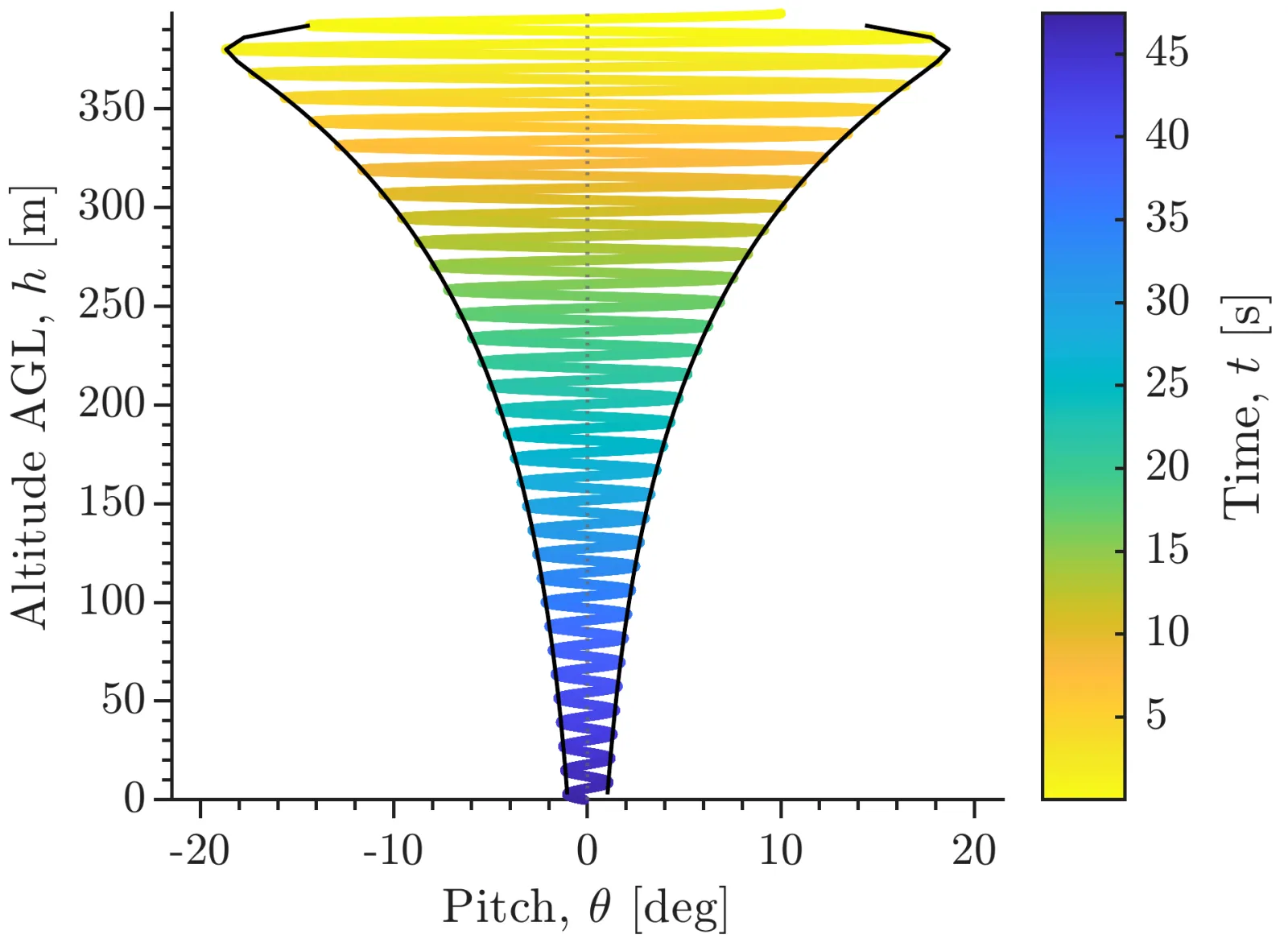
Pitch against altitude for the passive descent, a zigzag narrowing from plus and minus 19 degrees near 380 metres to almost vertical at the ground, coloured by time — Passive descent envelope: pitch against altitude, coloured by time.

Altitude falling linearly from 400 metres to zero over about 47 seconds, and vertical speed dropping from 40 metres per second to a flat 8.24 metres per second terminal velocity — Passive descent profile: altitude and vertical speed, terminal velocity 8.24 m/s.

Cumulative Monte-Carlo success rate against run count with a shaded confidence band, noisy below fifty runs and flat near 70 percent out to 300 — Cumulative success rate against run count with its confidence band, settling at 70 %. Why N=300 is enough.

The best landing

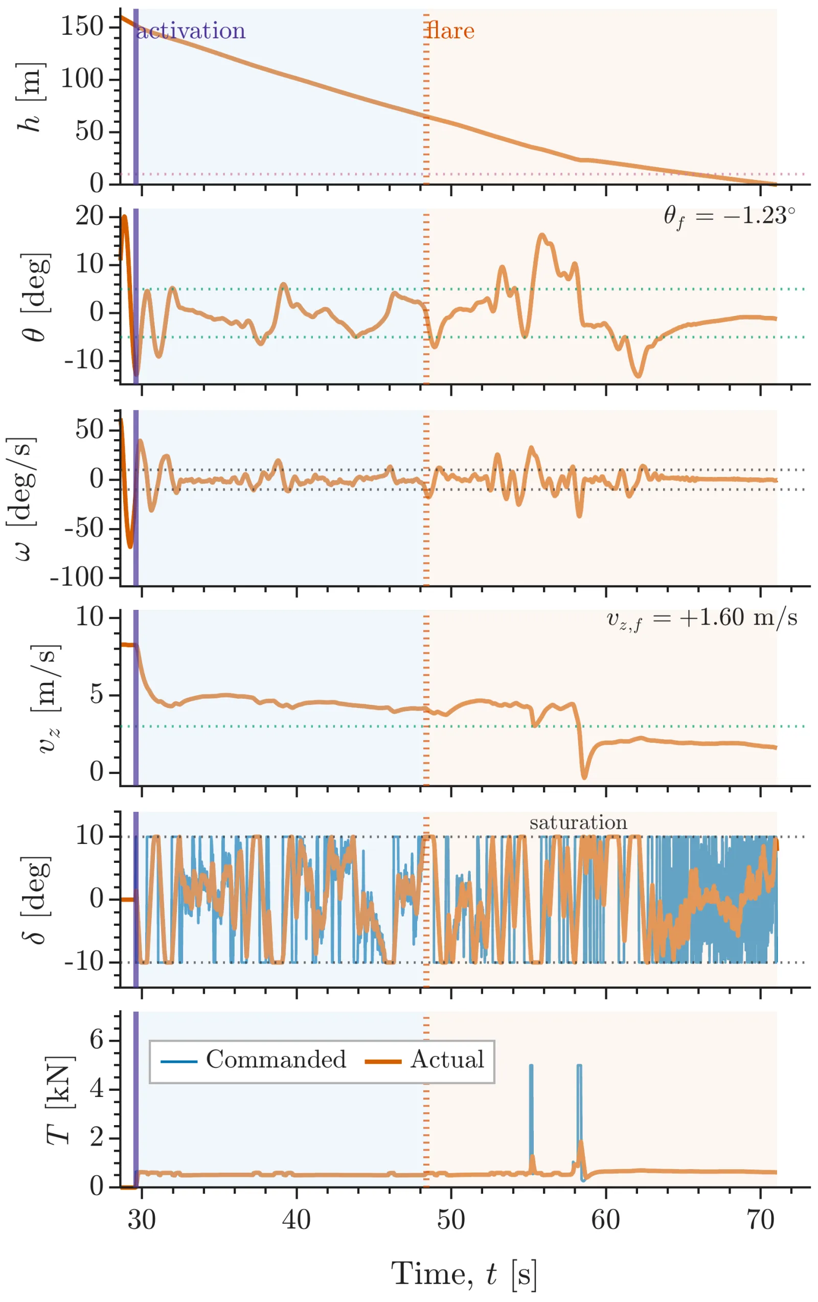
Run #59 is the one I would show a sceptic. The controller activates at 200 m with the vehicle still swinging through −25°, damps the oscillation, holds the descent near 4 m/s, then flares at 25 m to touch down at θ −0.63° and v_z 0.963 m/s. The gimbal sits on its ±10° limit for much of the flight, which says the actuator, not the control law, is the constraint. A representative median-grade run lands at −1.23° and 1.60 m/s, still inside the box, with two brief spikes to full thrust during the flare.

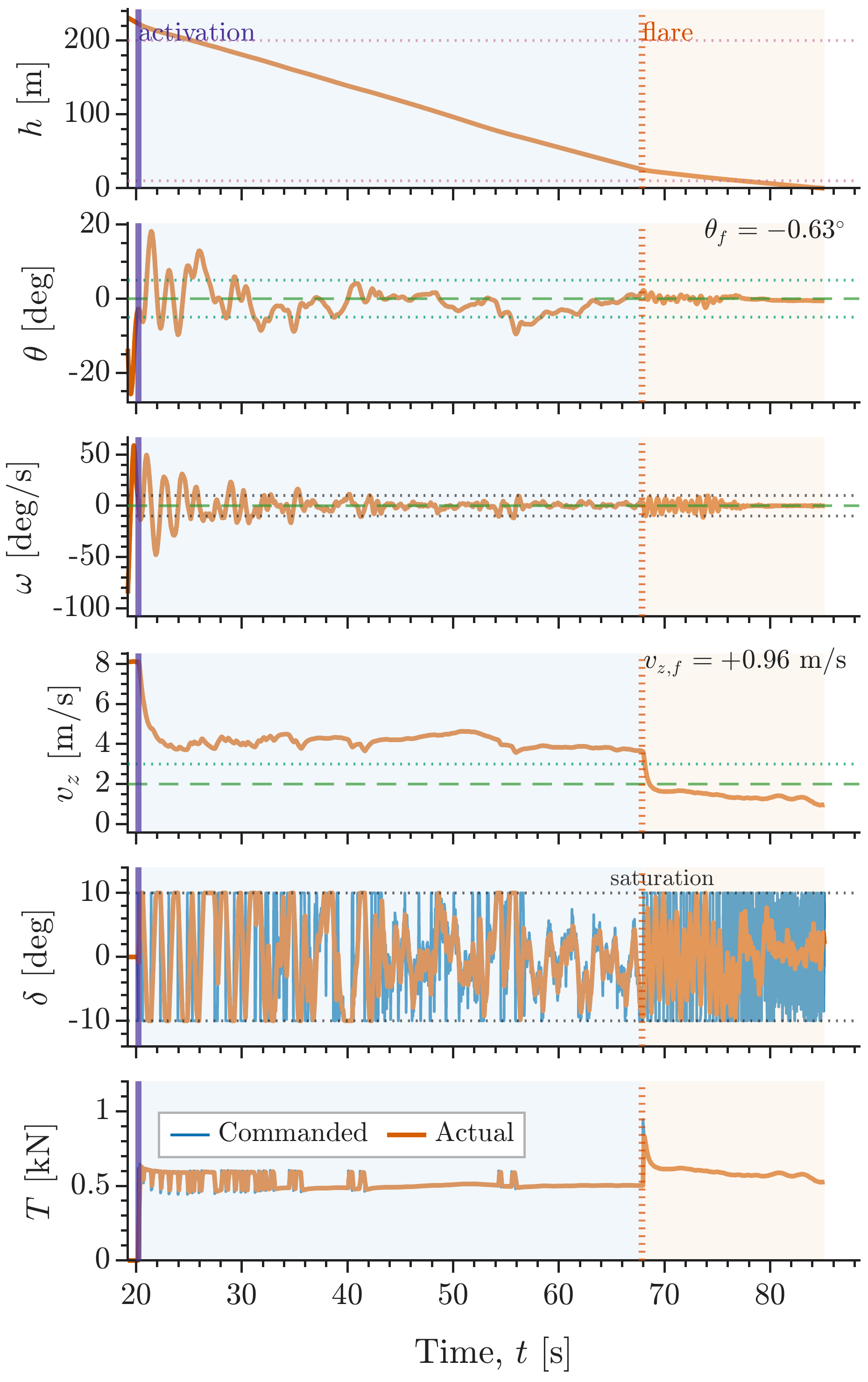
Six stacked time histories of a median-grade landing, pitch settling within a few degrees, descent speed stepping down at the flare, and two brief spikes to full thrust — A representative median-grade landing: θ −1.23°, v_z 1.60 m/s.

Where it fails

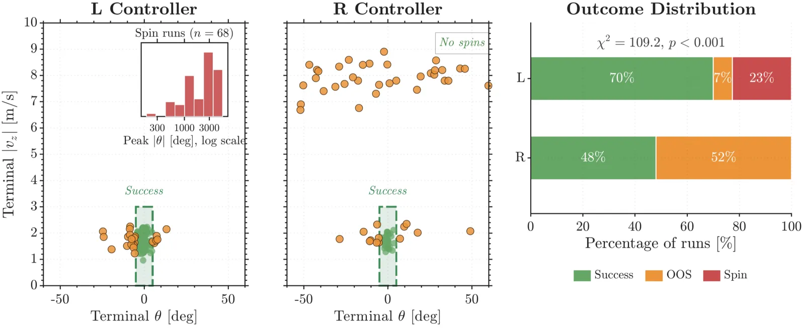
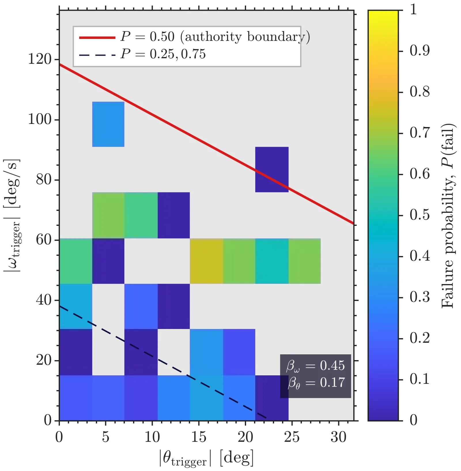
Failure is decided at the moment the controller arms. A logistic regression on the 300 trigger states puts the 50 % failure boundary at |ω_trigger| ≈ 119°/s: the rate matters (β_ω 0.45, p < 0.001) and the attitude barely does (β_θ 0.17, p = 0.221). That boundary is where the LQR linearisation stops describing the plant. I also ran a second controller, R, over 100 runs: 48 successes and 52 out-of-spec, χ² = 109.2 against L, p < 0.001. R records no spin-class landings, but that is a classification convention, not a raw result. Its failures cut thrust and ride the chute down at about 8 m/s, so they are counted as out-of-spec chute landings; the raw spin flag catches 31 of them.

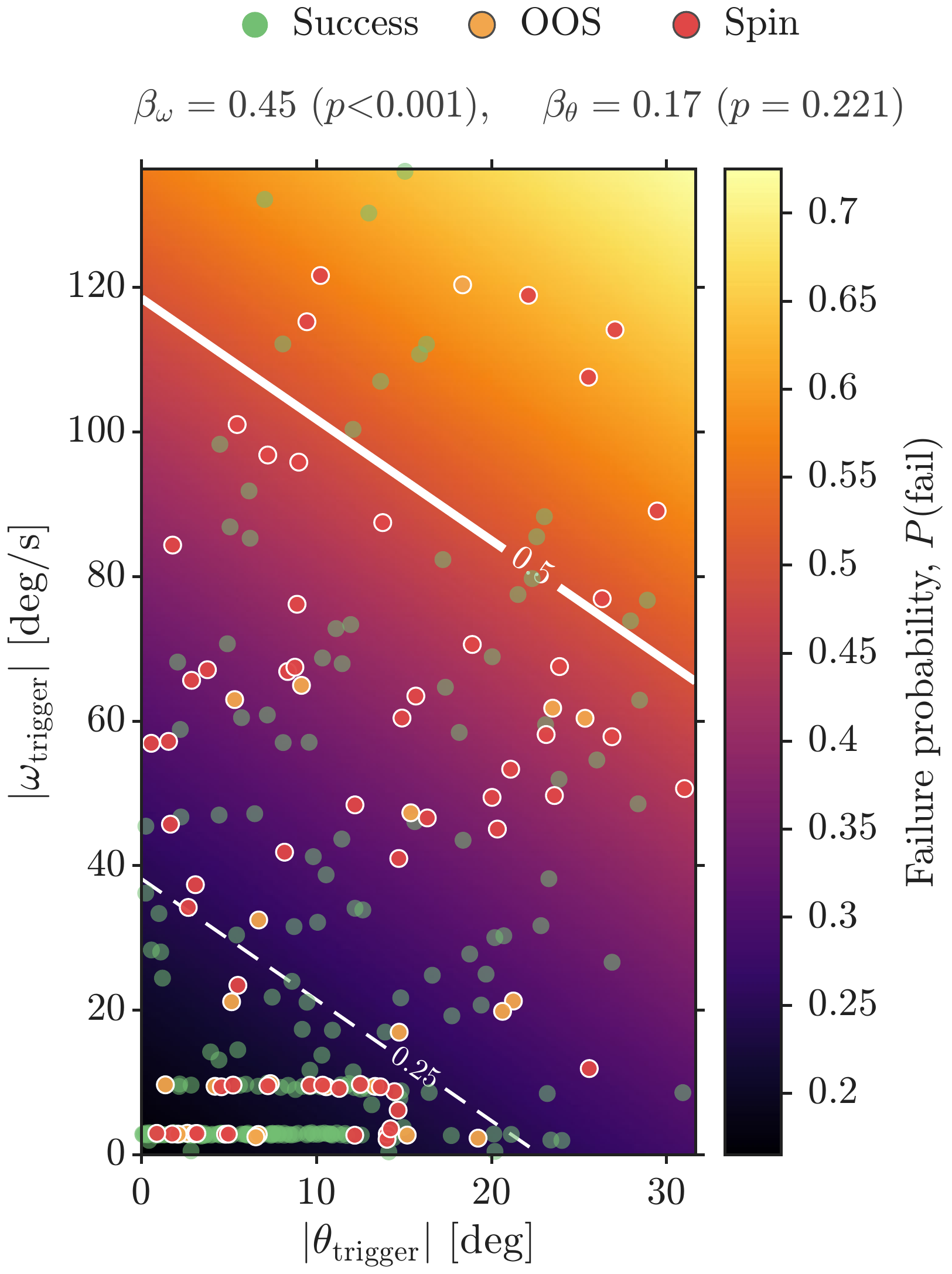
Heat-coloured failure-probability surface over trigger pitch and trigger rate with the 300 runs scattered on it, green successes, orange out-of-spec and red spins, and a white 0.5 contour crossing the rate axis near 119 degrees per second — Logistic failure-probability surface over trigger attitude and rate. P = 0.5 at |ω_trigger| ≈ 119°/s; β_ω 0.45 (p < 0.001), β_θ 0.17 (p = 0.221).

Binned failure-probability heatmap over trigger pitch and trigger rate, mostly blue at low rates and warming to yellow in the 45 to 60 degrees per second band, with a red P equals 0.5 authority boundary line — Failure probability binned over LQR-trigger states, with the P = 0.5 authority boundary.

Three panels: terminal speed against terminal pitch for the L controller with a cluster inside the success box, the same for the R controller with a band of out-of-spec landings near 8 metres per second, and stacked outcome bars for both — L against R: terminal-state scatter and outcome split, 70/7/23 % against 48/52/0 %. χ² = 109.2, p < 0.001. R's zero spins is a classification convention: its tumbles are counted as out-of-spec chute landings.

Fuel

Mean propellant over the campaign is about 12.6 kg, roughly a third of the ~40 kg a pure powered-descent-guidance landing of the same vehicle would need, because the chute does most of the braking for free. Flare height is the trade I tested: the 25 m flare the campaign flies costs 1.39 kg more than a 10 m flare (11.0 %, p = 0.003, 300 runs against 100). The 10 m case is the cheaper alternative I benchmarked against.

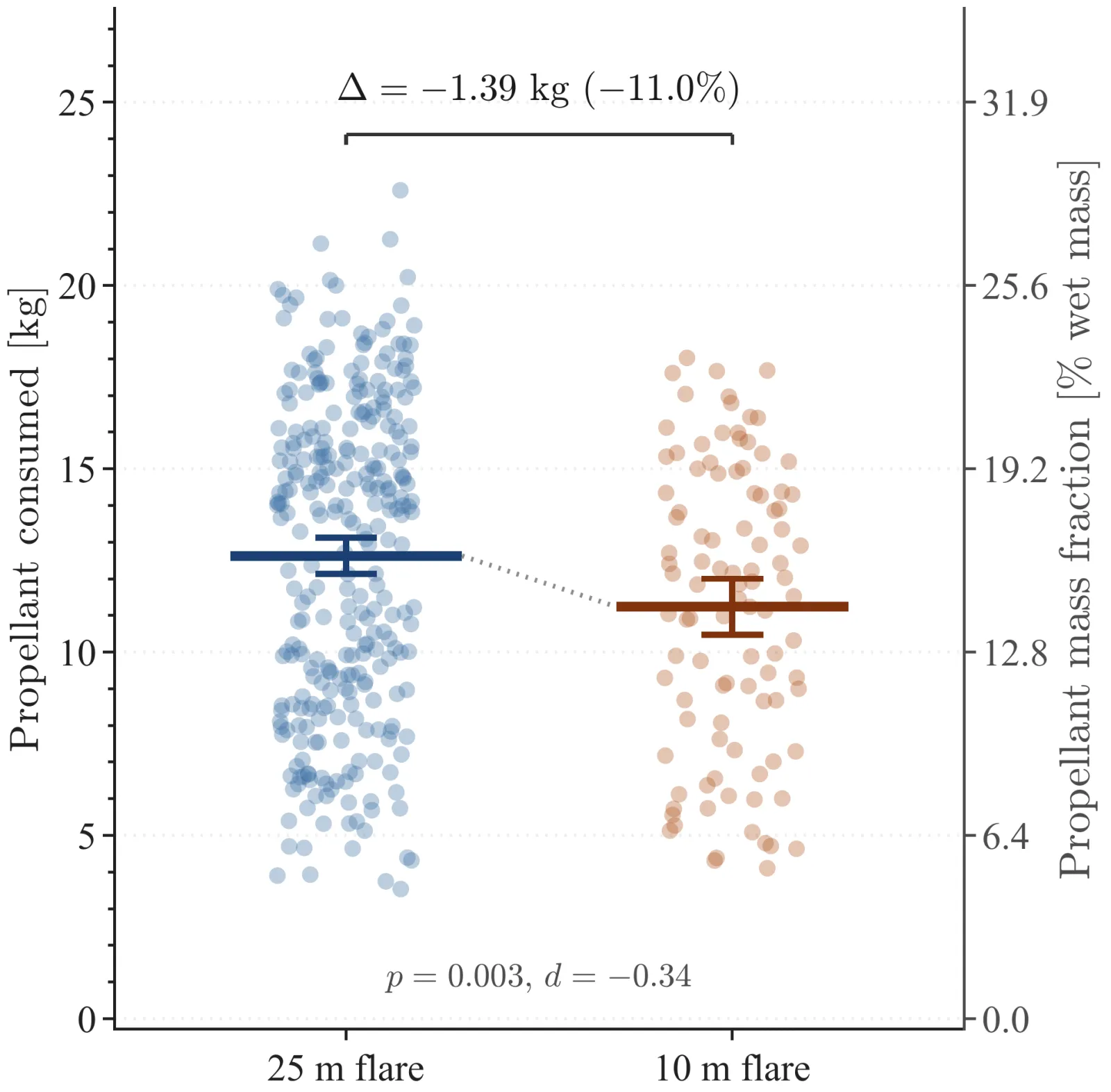
Propellant consumed per run as two dot swarms with mean bars, the 25 metre flare around 12.6 kilograms and the 10 metre flare lower, bracketed with a delta of minus 1.39 kilograms — Propellant consumed, 25 m against 10 m flare: −1.39 kg (11.0 %), p = 0.003.

Noise and turbulence

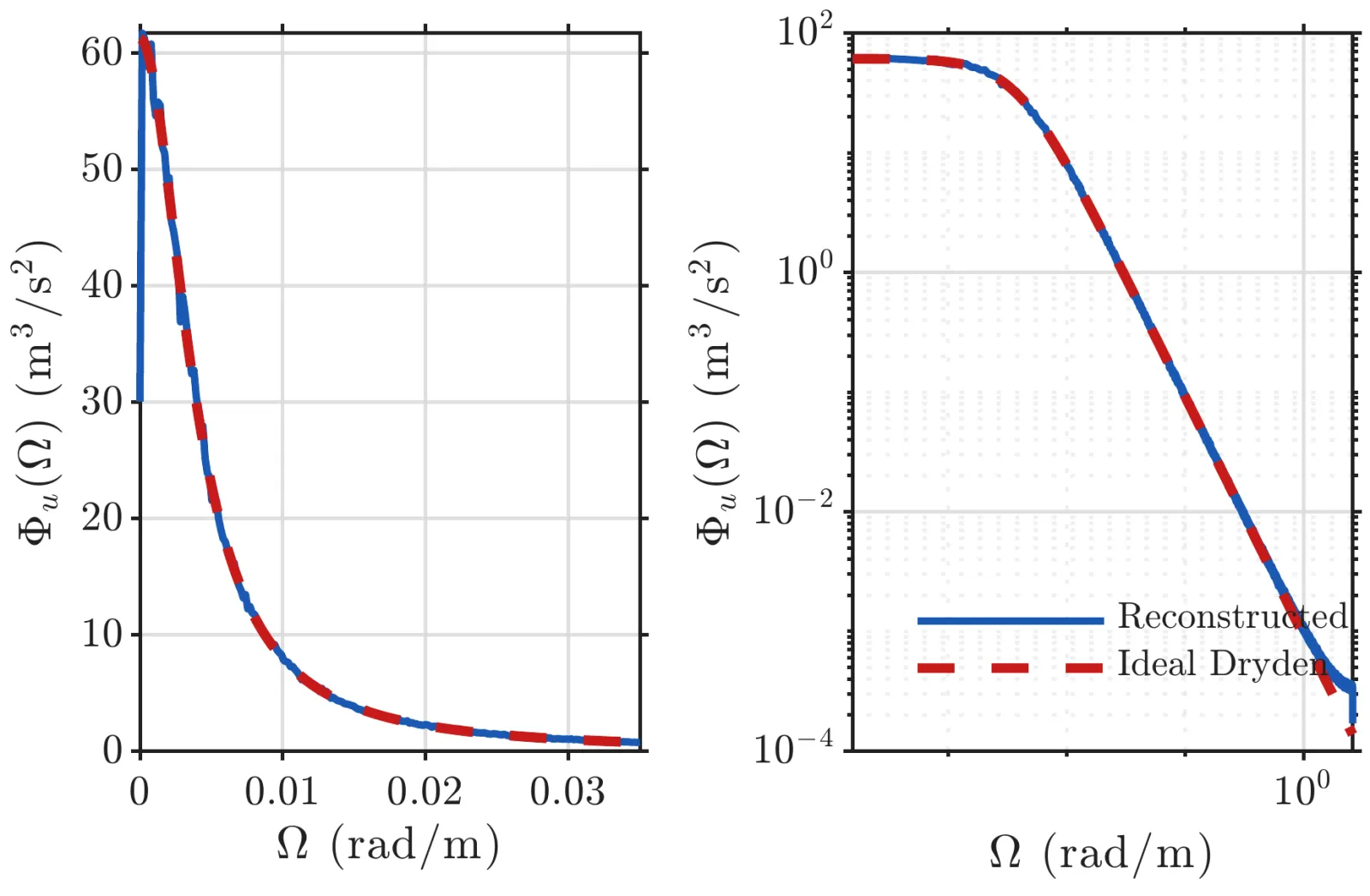
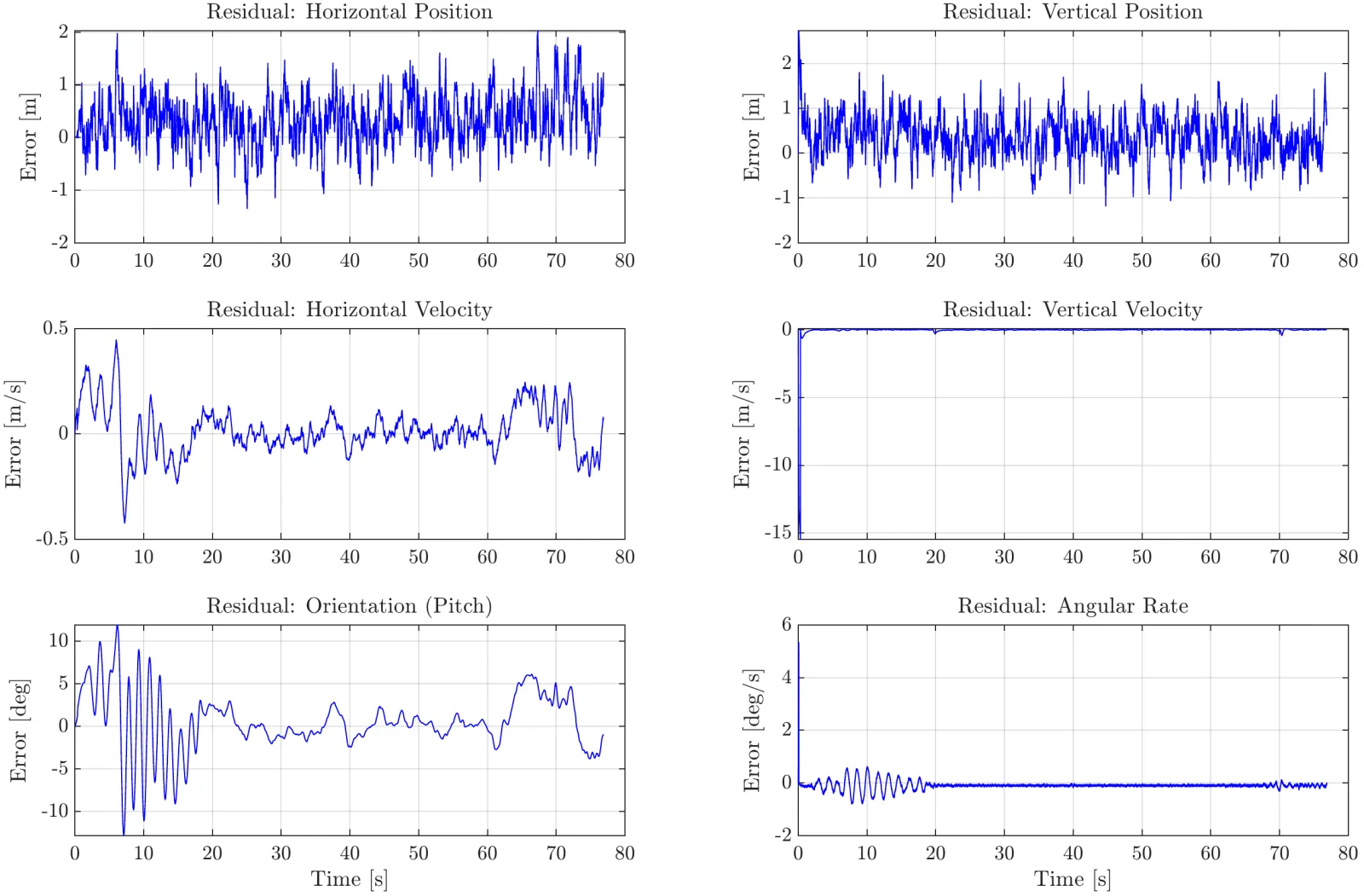
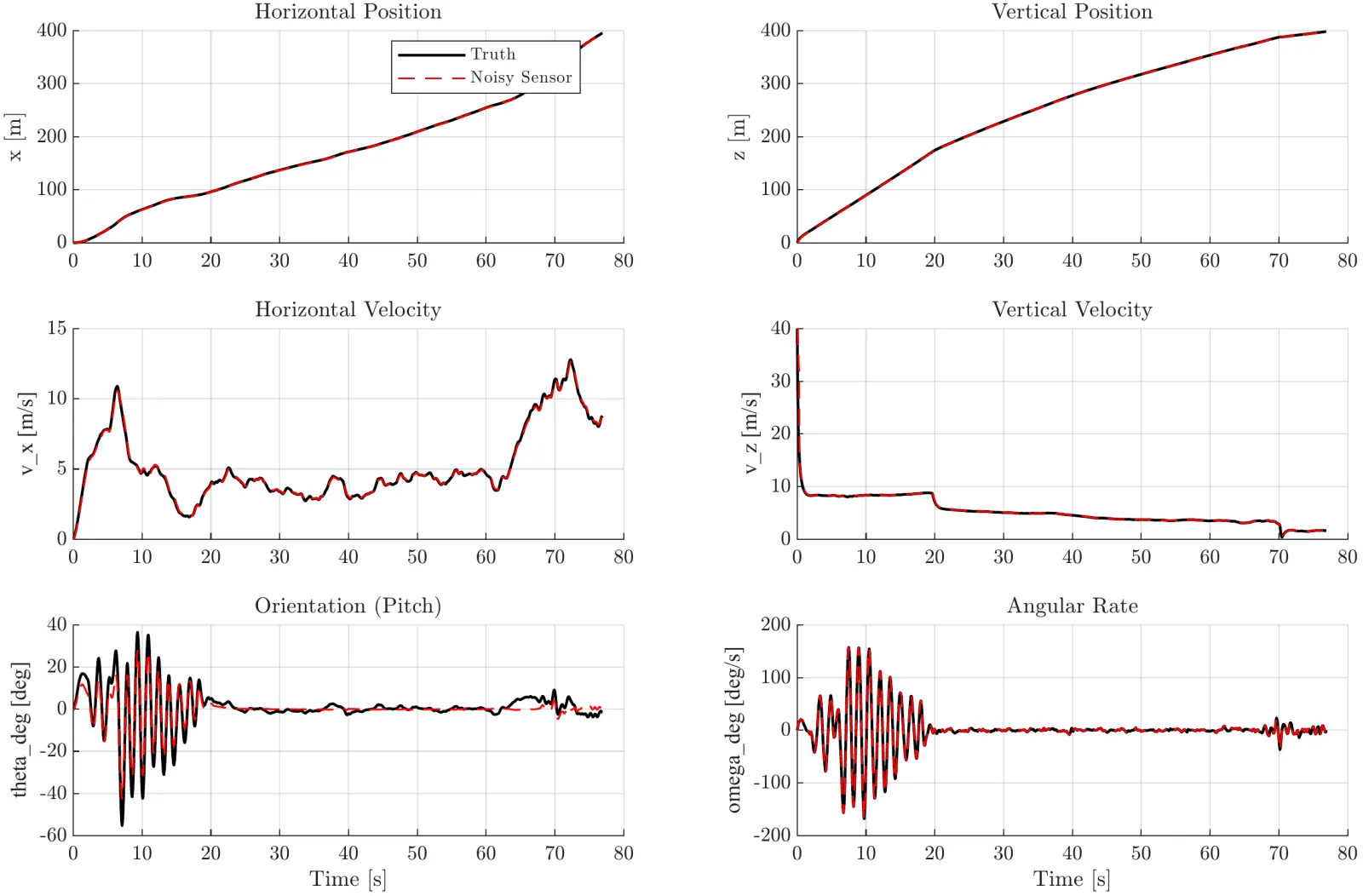
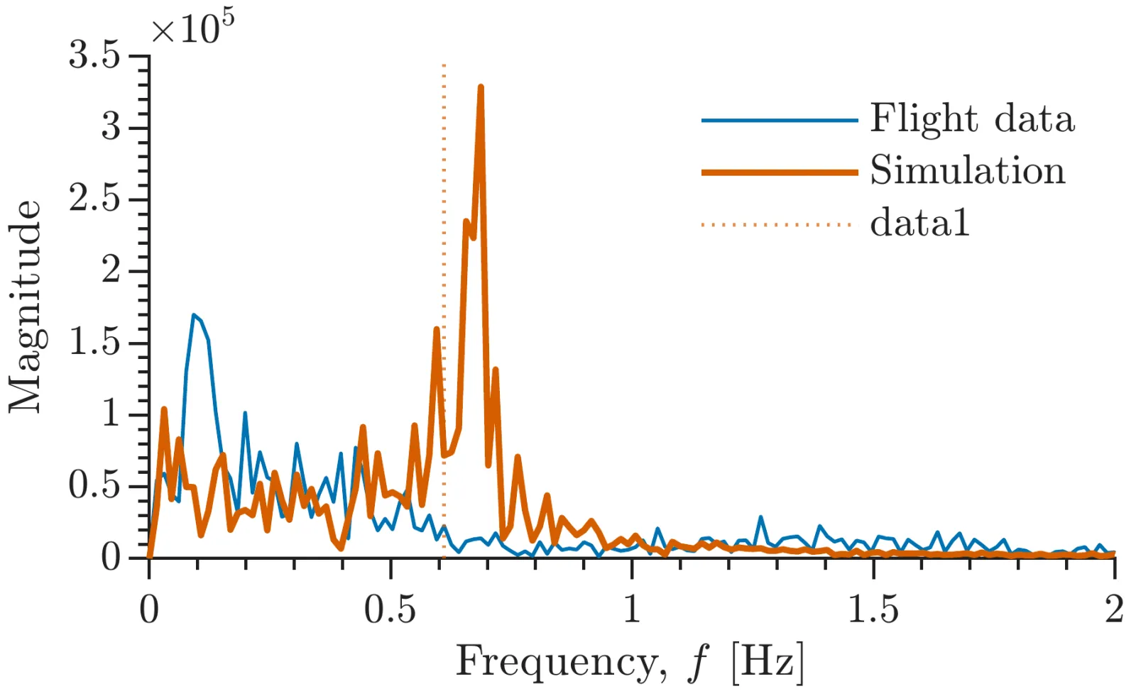
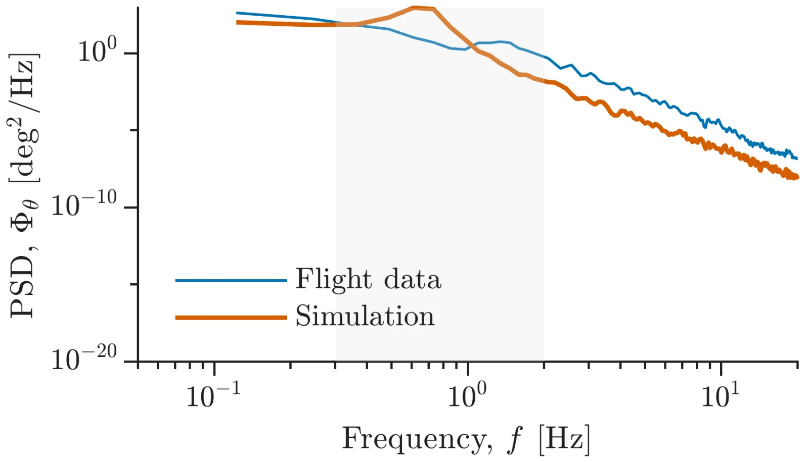
The atmosphere is log wind shear plus MIL-F-8785C gusts plus Dryden turbulence. I verified my Dryden filter against the NASA Langley LaSRS++ acceptance criteria; the reconstructed spectrum sits on the ideal curve on both linear and log axes. The plant was checked against BristolSEDS 6-DOF flight IMU tilt data: simulation and flight both concentrate their energy below 1 Hz, in the pendulum band. Sensors are modelled on a Murata SCH16T IMU and a u-blox MAX-M10S GPS, fused through a complementary filter; the residual plots show what the controller actually sees rather than the truth state.

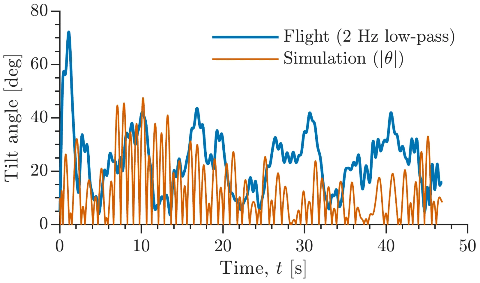
Tilt angle over 47 seconds, the low-passed flight record in blue and the simulated absolute pitch in orange, both swinging between roughly 0 and 45 degrees — Tilt angle, simulation against BristolSEDS flight IMU (2 Hz low-pass).

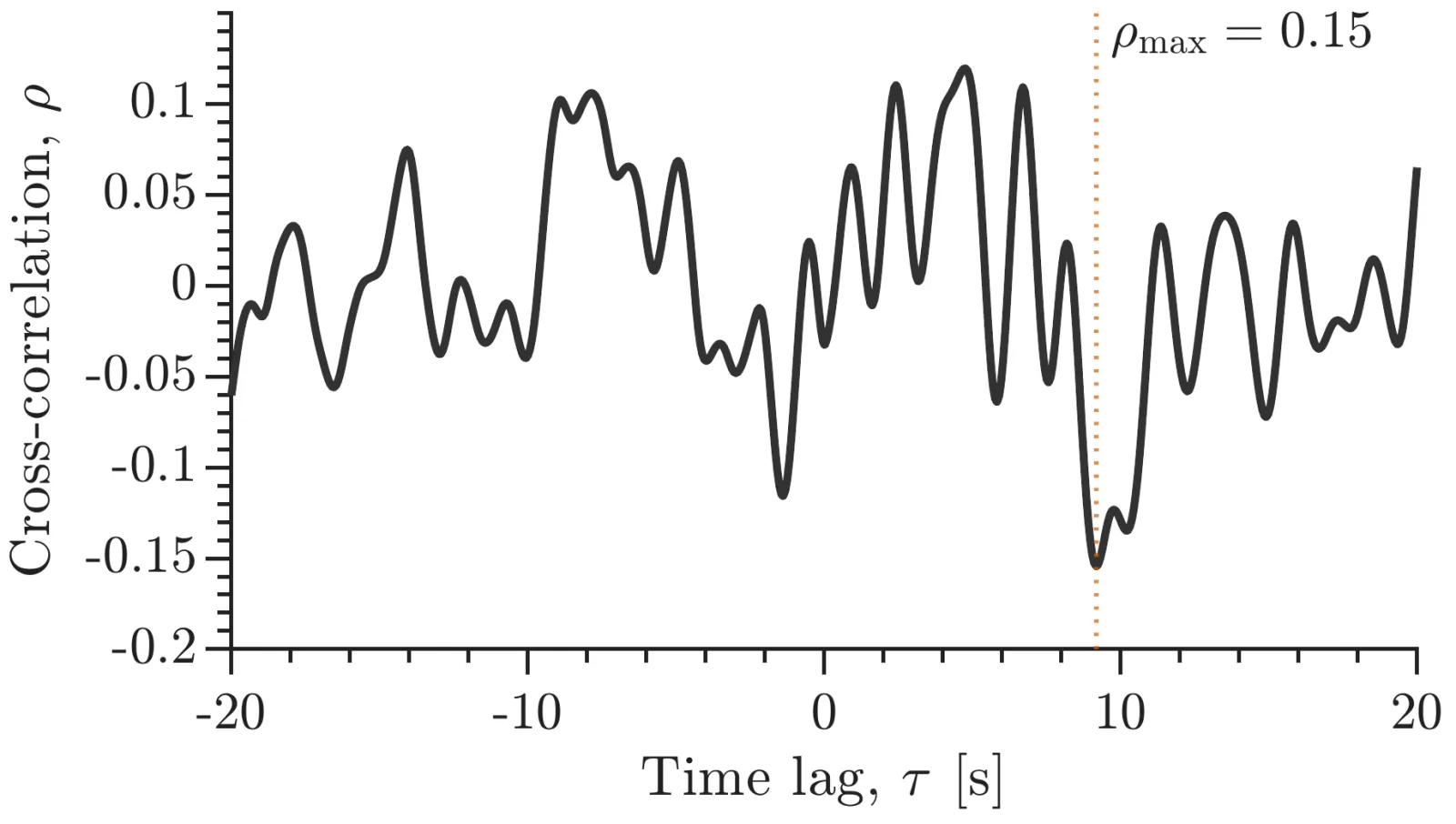
Cross-correlation between simulated and flight tilt against time lag from minus 20 to 20 seconds, staying within plus or minus 0.15 — Cross-correlation of simulated and flight tilt against time lag, ρ_max 0.15.

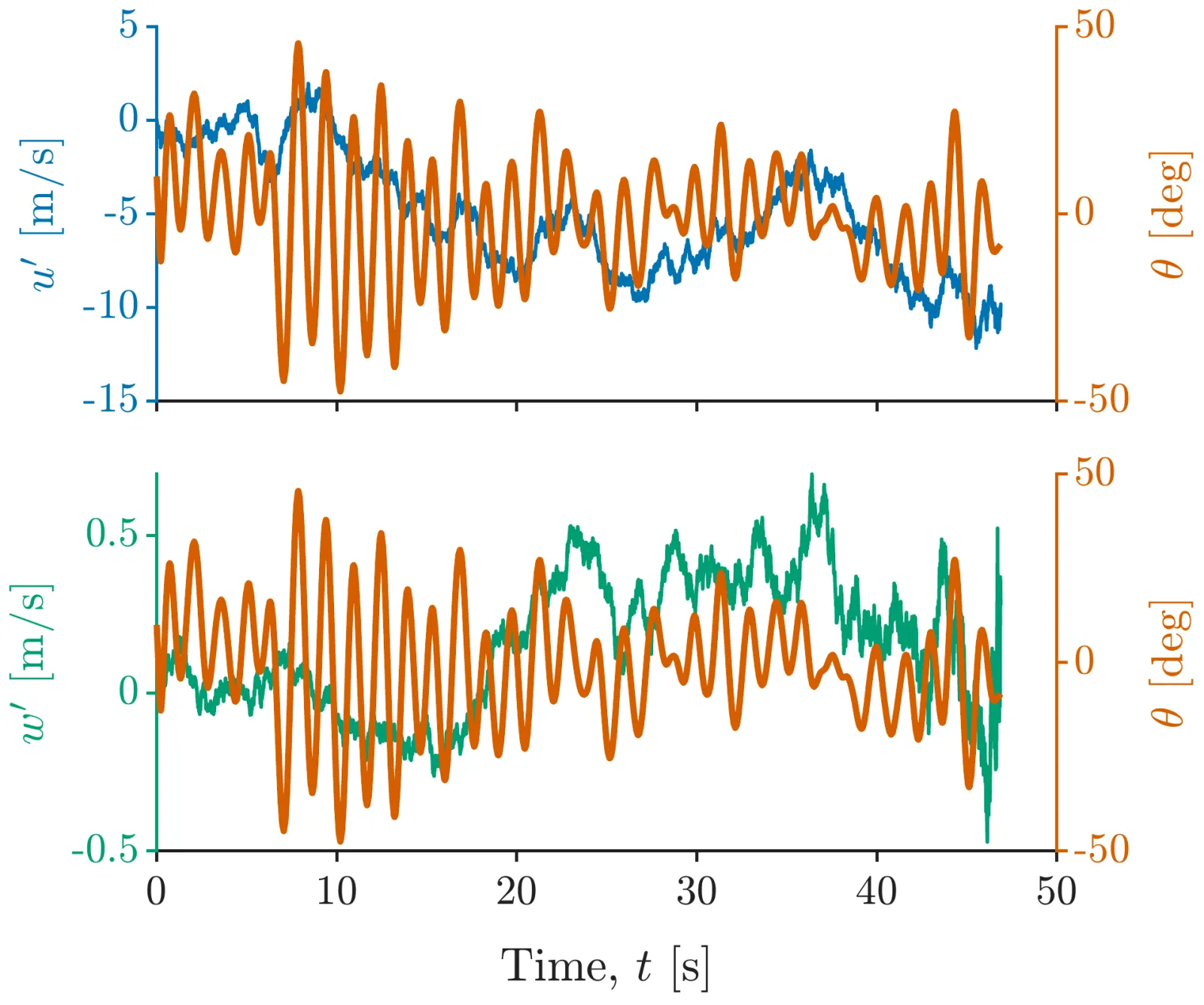
Two panels of pitch angle in orange overlaid on the horizontal and vertical turbulence components in blue and green over 47 seconds — Pitch response to the Dryden turbulence components u′ and w′.

Two plots of turbulence power spectral density against spatial frequency, linear and log-log, the reconstructed blue curve lying on the dashed red ideal Dryden curve — Dryden turbulence PSD, reconstructed against ideal, on linear and log axes. Verified against the NASA LaSRS++ acceptance criteria.

Six residual time histories from the sensor model: horizontal and vertical position, horizontal and vertical velocity, pitch and angular rate errors over 77 seconds — Sensor-model residuals: position, velocity, pitch and rate errors after the complementary filter.

Six state time histories with truth in black and the noisy sensor estimate dashed in red lying almost on top of it: positions, velocities, pitch and angular rate — Truth against noisy sensor estimates for the six states. Murata SCH16T IMU and u-blox MAX-M10S GPS models.

FFT magnitude of pitch against frequency from 0 to 2 hertz for flight data in blue and simulation in orange, both with their energy below 1 hertz — FFT of pitch, simulation against flight: both concentrate energy below 1 Hz.

Log-log power spectral density of pitch for flight data and simulation from 0.1 to 20 hertz with the pendulum band shaded — Pitch PSD, simulation against flight, pendulum band shaded.

Paper and poster

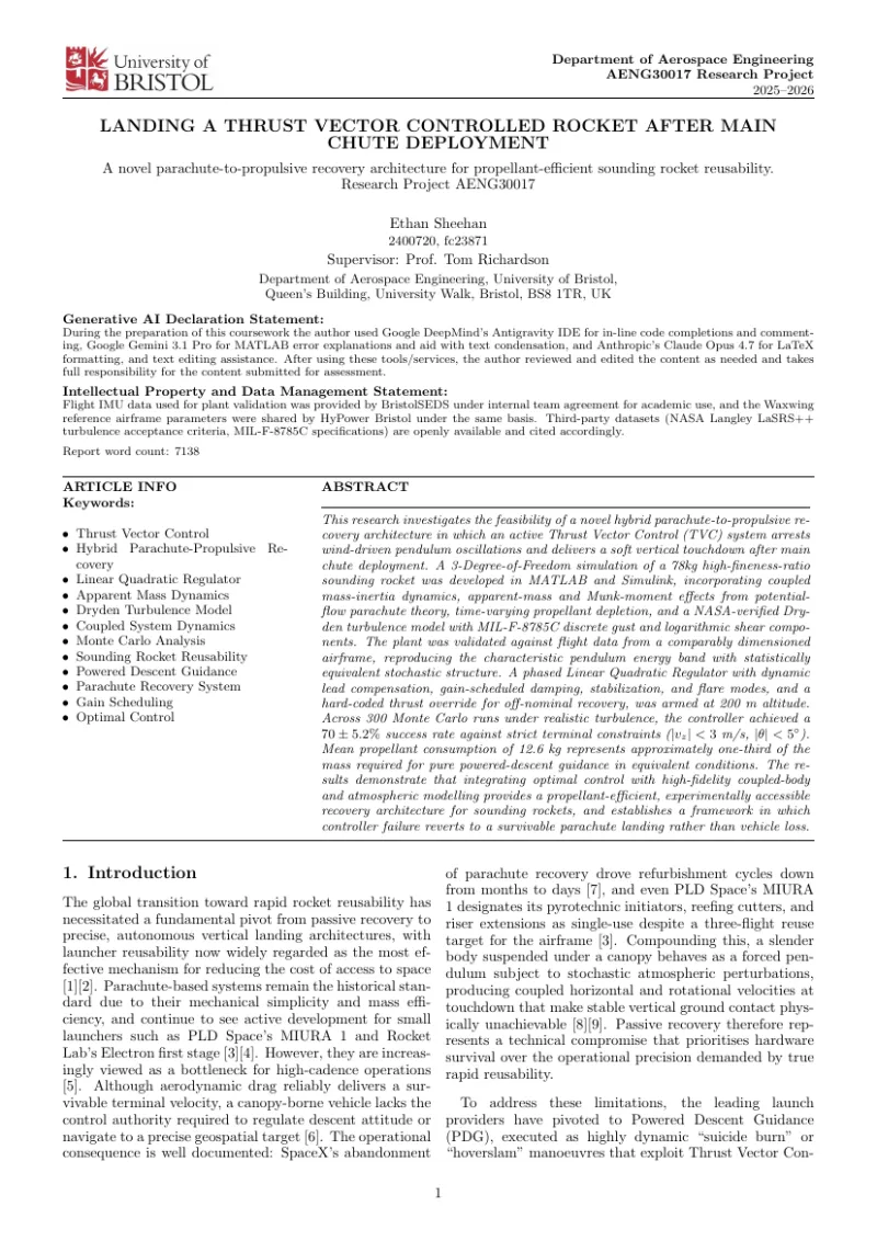
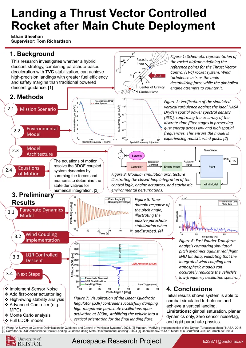
The full paper, 31 pages, compiled from the public repo. The conference poster was presented before the Monte-Carlo campaign existed: planar model, no sensor noise, preliminary results. It is here as the mid-project snapshot, not the final word. The engine lag model, the airframe and the validation data all come from the other projects on this site: BristolSEDS hotfires, HyPower's Waxwing, and the BristolSEDS flight IMU.

Landing a Thrust Vector Controlled Rocket After Main Chute DeploymentSubmitted paper, AENG30017, 2025-26.31 pp

Interim results posterInterim poster, presented before the Monte-Carlo campaign: planar model, no sensor noise, preliminary results.1 pp